Backpropagation through Poisson solvers
Continuing from the previous example this tutorial shows how to use automatic differentiaton with physics-inspired calculations. Let’s say we have a profile that can be parameterized by a free parameter. From this profile, we calculate another expression. And then we want to find the maximum of this expression as a function of the free parameter.
To be more precise, let’s say we have a quantity \(\rho\) with a profile that has a profile with a peak whose amplitude is parameterized by the parameter \(t\):
\[\begin{align} \rho_t(x) = -\sin^2(t) \exp \left( \frac{\left(x-x_0\right)}{2\sigma^2} \right) \times \frac{\sigma^2 - (x - x_0)^2}{\sigma^4} \end{align}\]The plot below shows how the peak of the amplitude varies with \(t\):
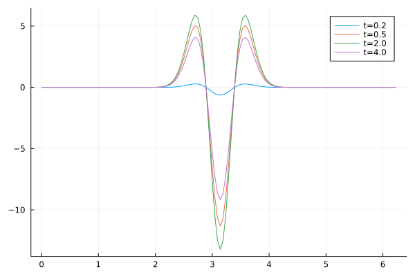
We see that for \(t = 0.2\ldots2.0\) the peak decreases in amplitude and increases as \(t\) increases from 2.0 to 4.0.
To complicate things a bit, we would like to know how a quantity that is derived from this profile depends on \(t\). In particular we want to
- Calculate \(\rho_t = \frac{\partial^2 \phi_t}{\partial x^2}\)
- Then maximize \(\int\limits_{0}^{L_x} \phi_t(x)^2 \, \mathrm{d}x\)
The ρ profile used here is after all a manufactured solution to the Poisson equation for
\[\begin{align} \phi_t(x) = \sin^2(t) \exp \left( \frac{\left(x-x_0\right)}{2\sigma^2} \right). \end{align}\]Then we only have to ask Wolfram Alpha to give us
\[\begin{align} I(t) = \int \limits_{0}^{L_x} \phi_t(x)^2 = \frac{\sqrt{2 \sigma} \sin(t)^4}{s} \left[ \mathrm{erfi}\left( \frac{L-x_0}{\sqrt{\sigma}} \right) + \mathrm{erfi}\left( \frac{x_0}{\sqrt{\sigma}}\right)\right]. \end{align}\]But in this tutorial the focus is on using automatic differentiation for such tasks. In particular, we can use the approach presented here when we lack an analytic solution for ϕ. We can also use the approach presented here when we lack an analytic expression for ρ, as long as we can generate ρ given a value for t.
So let’s draft a game-plan. First we choose a discretization of the domain [0:Lx] using Nx grid points, equidistantially spaced with \(\triangle x\). Then we pick a value of t and
- Calculate \(\rho_t(x)\).
- Invert the poisson equation to find \(\phi_t(x)\).
- Calculate the integral \(I(t) = \int \phi_t(x)^2 \mathrm{d}x\).
Starting it off, we import relevant libraries, in particular Zygote, and define parameters for the grid and the profile:
using Zygote
using FFTW: fft, ifft
using LinearAlgebra
using BenchmarkTools

Lx = 2π
Nx = 128
Δx = Lx / Nx
n0 = 0.0
μ = π
σ = 0.25
t = 1.0
Since we later ask for the \(\partial_t I(t)\) we write a function that calculates \(I(t)\):
function int_prof(t)
    # This calculates I(t)
    xrg = Δx * (0:1:(Nx-1))
    ρ = ρ_prof(xrg, 1.0, t, μ, σ)
    ϕ = invert_poisson(ρ, Nx, Lx)
    ϕ = ϕ .- mean(ϕ)
    sum(ϕ.^2)
end
That’s it. Now we can call Zygote’s gradient function on int_prof(t) to take calculate
\(\partial_t I(t)\). Now there are some more details to explore. In the next section
we digress into Poisson solvers. Feel free to skip this section and head straight to
the results to see how well AD performs on this relatively simple forward model.
Poisson Solvers
Given \(\rho_t\), we want to solve the Poisson equation
\[\begin{align} \rho_t(x) & = \frac{\partial^2 \phi_t)x)}{\partial x^2} \\ \phi_t(0) & = \phi_t(L) \end{align}\]for \(\phi_t\) on the domain \(x \in [0:L]\). We don’t even pretend that we have any class and use periodic boundary conditions. We want the solution on the grid points \(x_i = i \triangle x\), where \(\triangle x = L_x / N_x\) and \(N_x\) denotes the number of grid points.
For this task wwe can either follow this excellent tutorial or use a spectral solver, described for example here.
A simple spectral solver for can be implemented like this:
# Simple spectral solver for Laplace equation
function invert_laplace_spectral(y::Array{Float64}, Nz, Lz)
    k = [1e100; 1:(Nz ÷ 2); -(Nz ÷ 2 - 1):-1] .* 2π/Lz
	y_ft = -fft(y) ./ k ./ k
    y_ft = y_ft .* [0; ones(Nz - 1)]
    d2y = real(ifft(y_ft))
end
The first line assembles a vector of wave numbers. The solution to Poisson’s allows an arbitrary offset. Setting the element of the
wave numbers vector, that corresponds to the zero frequency, to a large number
, k[1] = 1^100, we fix the mean of the solution to zero since we later divide by k.
We then take the Fourier transformation, divide by \(k^{2}\) and explicitly
zero out the zero-mode. The syntax is a bit cumbersome, we perform a point-wise
multiplication with an array, since Zygote does not support array mutation.
Finally we take the real part of the inverse transformation.
A particlar issue with Zygote is that it can’t handle code that mutates arrays. The following text snippet shows a way of how to assemble an array and a way that will fail:
[0; ones(Nz - 1)]   # This will work with Zygote

tt = ones(Nz)
tt[1] = 0           # This will not work with Zygote
Alternatively, we can implement a finite difference solver for Poisson’s equation. Below is the implementation for periodic boundary conditions adapted from herel
function invert_laplace(y,  Nz, Lz)
    Δz = Lz / Nz
    invΔz² = 1.0 / Δz / Δz

    A0 = Zygote.Buffer(zeros(Nz, Nz))
    for n ∈ 1:Nz
        for m ∈ 1:Nz
            A0[n,m] = 0.0
        end
    end
    for n ∈ 2:Nz
        A0[n, n] = -2.0 * invΔz²
        A0[n, n-1] = invΔz²
        A0[n-1, n] = invΔz²
    end
    A0[1, 1] = 1.0
    A0[1, 2] = 0.0
    A0[Nz,1] = invΔz²

    A = copy(A0)
    yvec = vcat([0.0], y[2:Nz])
    ϕ_num = A \ yvec
end
After calculating sample spacing, the code constructs a Matrix for the finite difference Laplace operator. Here we use Zygote.Buffer which allows us to use array mutation syntax. Again, code that is to be differentiated with Zygote can’t mutate arrays. After assembling the matrix we copy it into a matrix, augment the input vector and solve the linear system.
Differentiation through Poisson solvers
The code below shows how I set up the problem. I choose \(\phi\) and
\(\rho\) as a manufactured solution. This way I can compare the
numerical solution for \(\phi_t\) to ϕ_prof. A Gaussian solution is
also a craving test case for a spectral solver. Since the Fourier
transformation of a Gaussian is a Gaussian, all Fourier modes will be
non-negative. This way one can pick up errors where a mode is at a wrong
place in an array.
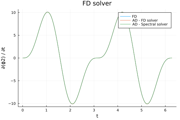
The functions int_prof_fd(t) and int_prof_sp(t) implement the three
prong workflow described above. In particular their only argument is t.
This way we can pass the whole workflow to Zygote.gradient and this way
get the derivative of I with respect to t, $$\partial_t I$.
Now let’s set up the code:
ϕ_prof(xrg, n0, t, μ, σ) = n0 .+ sin(t).^2 .* exp.(-(xrg .- μ).^2 ./ 2.0 ./ σ ./ σ)
ρ_prof(xrg, n0, t, μ, σ) = -sin(t)^2 * exp.(-(xrg .- μ).^2 / 2 / σ / σ) .* (σ^2 .- (xrg .- μ).^2) / (σ^4)

Lx = 2π
Nx = 128
Δx = Lx / Nx
n0 = 0.0
μ = π
σ = 0.25
t = 1.0

function int_prof_fd(t)
    xrg = Δx * (0:1:(Nx-1))
    ρ = ρ_prof(xrg, 1.0, t, μ, σ)
    ϕ = invert_laplace(ρ, Nx, Lx)
    ϕ = ϕ .- mean(ϕ)
    sum(ϕ.^2)
end

function int_prof_sp(t)
    xrg = Δx * (0:1:(Nx-1))
    ρ = ρ_prof(xrg, 1.0, t, μ, σ)
    ϕ = invert_laplace_spectral(ρ, Nx, Lx)
    sum(ϕ.^2)
end

trg = 0.0:0.01:2π
phi2_fd = zeros(length(trg))
phi2_sp = zeros(length(trg))

phi2_grad_fd = zeros(length(trg))
phi2_grad_sp = zeros(length(trg))

for idx ∈ 1:length(trg)
    t = trg[idx]
    phi2_fd[idx] = int_prof_fd(t)
    phi2_grad_fd[idx] = gradient(int_prof_fd, t)[1]

    phi2_sp[idx] = int_prof_sp(t)
    phi2_grad_sp[idx] = real(gradient(int_prof_sp, t)[1])
end
As a sanity check we first compare the output of the forward model when using the finite difference and spectral solver.
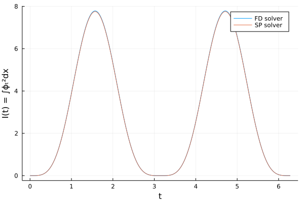
For the resolution I chose, \(\triangle x\) is approximately 0.5 in this example, both solvers perform well.
A final thing to look at is speed. Using Benchmarktool we can evaluate the performance of backpropagating through either the finite difference and the spectral solver:
using BenchmarkTools
julia> @benchmark gradient(int_prof_sp, t)[1]
BenchmarkTools.Trial:
  memory estimate:  141.64 KiB
  allocs estimate:  752
  --------------
  minimum time:     110.582 μs (0.00% GC)
  median time:      118.785 μs (0.00% GC)
  mean time:        139.315 μs (9.20% GC)
  maximum time:     12.583 ms (68.76% GC)
  --------------
  samples:          10000
  evals/sample:     1

julia> @benchmark gradient(int_prof_fd, t)[1]
BenchmarkTools.Trial:
  memory estimate:  6.07 MiB
  allocs estimate:  170758
  --------------
  minimum time:     28.093 ms (0.00% GC)
  median time:      32.338 ms (0.00% GC)
  mean time:        35.562 ms (3.07% GC)
  maximum time:     104.050 ms (0.00% GC)
  --------------
  samples:          141
  evals/sample:     1
The mean time it takes to backprop through the finite difference solver is about 250 times larger than for the spectral solver. Given that the spectral solver is cheaper to evaluate, it doesn’t require to solve a linear system, this is not completely unexpected.