Backpropagation through numerical calculations

Differentiable programming makes all code amenable to gradient based optimization. This harmless statement has broad implications. Think for example about a physical simulation where a differential equation is integrated in time. Given some initial conditions, boundary conditions, and parameters, the simulator approximates how the system evolves in time. Now lets say you simulate a wave in a swimming pool that moves towards a wall. Your goal is to find out how fast the wave has to be launched as to swap over the edge it is travelling to. With differentiable programming, you could define a target metric and optimize it with respect to the initial condition, here the speed with which the wave is launched.

To get started with differentiable programming we are looking at a very simple example. We are given a density profile n on a finite domain:

\[\begin{align} n(z) = n_0 + \sin(t) \exp\left( \frac{z-z_0}{2\sigma}\right). \end{align}\]

The background density is \(n_0\) on which a Gaussian density peak, centered around \(z_0\) modulated. The amplitude of the peak is given by \(\sin(t)\). And we are interested on how the integral of the profile over the domain varies with t. Of course this can be calculated analytically:

\[\begin{align} \int \limits_{-L_z}^{L_z} n(z')\, \mathrm{d}z' = L_z n_0 + \sin(t)^2 \sqrt{2\pi} \sigma \mathrm{erf} \left( \frac{1}{\sqrt{2}\sigma} \right) \end{align}\]

To study the dependence of this integral on the amplitude parameter t we evaluate the derivative:

\[\begin{align} \frac{\partial N}{\partial t} = L_z \sqrt{2\pi} \sigma \mathrm{erf}\left( \frac{1}{\sqrt{2}\sigma} \right) \sin(t) \cos(t). \end{align}\]

To find the amplitude t that maximizes N we can now just set \(\partial N/\partial t = 0\) and solve for t. But in a situation where we are not so lucky and have an analytic expression we may want to use automatic differntiation. Let’s do this in Julia.

Automatic differentiation in Julia

First things first - import Zygote to do automatic differentiation and the plots package as well as the error function erf:

using Zygote
using Plots
using SpecialFunctions: erf

Now we define a function that gives our density profile:

gen_prof(xrg, n0, t, z0, σ) = n0 .+ sin(t).^2 .* exp.(-(zrg .- z0).^2 ./ 2.0 ./ σ ./ σ)

For automatic differentiation to do its magic we need to numerically integrate the profile.

function int_prof(t)
    my_prof = gen_prof(z0:Δz:z1, n0, t, μ, σ)
    my_sum = sum(my_prof) * Δz
end

This function generates a vector which holds values of the profile at the points starting at \(z_0\) to \(z_1\), spaced regularly with \(\triangle z\). The parameters \(\mu\) and \(\sigma\) are captured from the context where the function is called from later. After generating the profile vector we numerically integrate the profile using the rectangle rule.

Now we have all the ingredients to calculate \(\partial N/\partial t\) using automatic differentiation. In code, we first define the necessary parameters and allocate vectors for the t’s where we want the derivative:

n0 = 1.0
σ = 0.2
x0 = -1.0
x1 = 1.0
Δx = 0.01
n0 = 1.0
μ = x0 + (x1 - x0) / 2.0
σ = (x1 - x0) / 10.0

# Perform numerical integration of the profile for a range of t's:
t_vals = 0.0:0.05:6.5
sum_vals = similar(t_vals)
sum_vals_grad = similar(t_vals)

To find the gradient, we first evaluate int_prof for a given value of t. Then we call gradient(int_prof, t) on this call. The return value is just the gradient \(\partial N / \partial t\). Thist functionality is just Zygote’s gradient doing it’s work but on a more complicated example than in the documentation. Note that gradient returns a tuple where the actual gradient is the first element.

for tidx ∈ tvals
    t = t_vals[tidx]
    sum_vals[tidx] = int_prof(t)
    sum_vals_grad[tidx] = gradient(int_prof, t)[1]
end

The gradient calculated using automatic differentiation can be compared to the analytic formula:

dNdt_anl = 2. * sqrt(2π) * σ .* sin.(t_vals) .* cos.(t_vals) .* erf(1 / √(2) / σ )

p = plot(t_vals, sum_vals_grad, label="∂ ∫n(z,t) dz / ∂t (autodiff).")
plot!(p, t_vals, dNdt_anl, label="∂ ∫n(z,t) dz / ∂t(analytical).", xlabel="t")

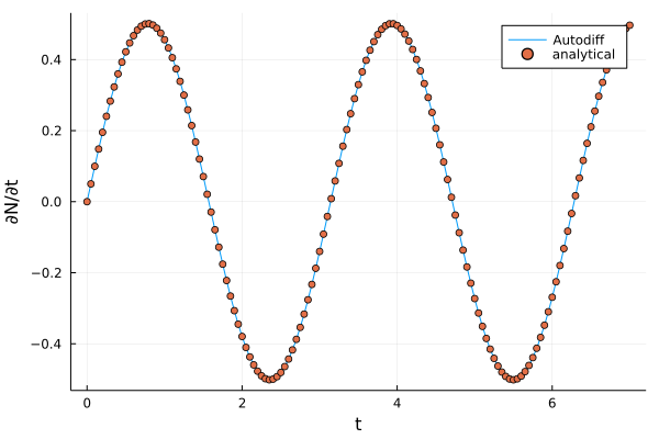
As shown in the plot, the analytical derivative and the one calculated by automatic differentiation are almost identical.

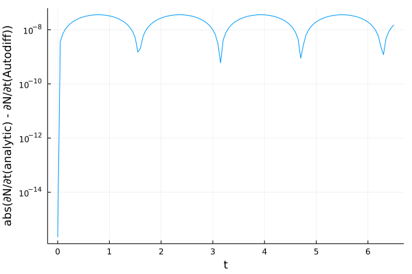
And plotting the error, we find differences of the order of \(10^{-8}\) to \(10^{-9}\).

Summary

In this blog post we looked at a very simple use-case for automatic differentiation. We have a mathematical expression that we know depends on a paramter and we wish to find the optimum value of this expression. Using automatic differentiation we now can calculate the gradient of that expression with respect to the parameter. This approach allows one to find the optimize the expression with resepct to the value.

A common procedure for this optimization is gradient descent, used in deep learning. Instead of a optimizing a neural network, automatic differentiation can be applied to arbitrary code. So we can optimize a much broader class of items than just neural networks.