Automatic differentiation - Reverse Mode

This post is the follow-up of my post on forward mode AD. There I motivated motivated the use of automatic differentiation by noting that it is helpful for gradient-baseed optimization. In this post I will discuss how reverse mode allows us to take the derivative of a function output with respect to basically an arbitrary number of parameters in one sweep. To do this comfortably, one often evaluates local derivatives, whose use is facilitated by introducing the bar notation.

To see this, let’s go the other way around. Given our computational graph we start at the output $yy$ and calculate derivatives with respect to intermediate values. For convenience we define the notation

$$\begin{align} \bar{u} = \frac{\partial y}{\partial u} \end{align}$$

that is, the symbol under the bar is the variable we wish to take the derivative with respect to. Now let’s dive right in and take derivatives from the example. We start out with

$$\begin{align} \bar{v}_6 & = \frac{\partial y}{\partial v_6} = 1 \\ \bar{v}_5 & = \frac{\partial y}{\partial v_5} = \frac{\partial y}{\partial v_6} \frac{\partial v_6}{\partial v_5} = \bar{v}_6 \frac{\partial v_6(v_4, v_5)}{\partial v_5} = \bar{v}_6 v_4 \\ \end{align}$$

The first expression is often called the seed gradient and is trivial to evaluate. In order to evaluate $\bar{v}_5$ we had to use the chain-rule.

Continuing, we now have to evaluate $\bar{v}_4$. Let’s do it first using the chain rule:

$$\begin{align} \frac{\partial y}{\partial v_4} & = \frac{\partial y}{\partial v_6} \left( \frac{\partial v_6}{\partial v_5} \frac{\partial v_5}{\partial v_4} + \frac{\partial v_6}{\partial v_4} \right) \\ & = v_4 (-1) + v_5. \end{align}$$

where we have used the chain rule and that $v_6 = v_6(v_5(v_4), v_4)$. Looking at the computational graph, we see that we had to split the product using a plus-sign precisely at a position where there are multiple paths from the origin $y$ to the target node $v_4$, one via $v_6$ and one via $v_5$. Now as trivial as this example is, real-world programs are often much more complicated. And to calculate the partial derivatives, the formulas can become ever more complex.

Now the bar notation is here to make our life easier. Essentially, it gives us an easy way to replace chain-rule evaluation with local values that are stored in all child-nodes of the target node $v_i$ in $\bar{v}_i$. Put in another way, they are used as cache-values when traverseing the graph from right-to-left, as we do in reverse-mode AD. This is illustrated in the sketch below:

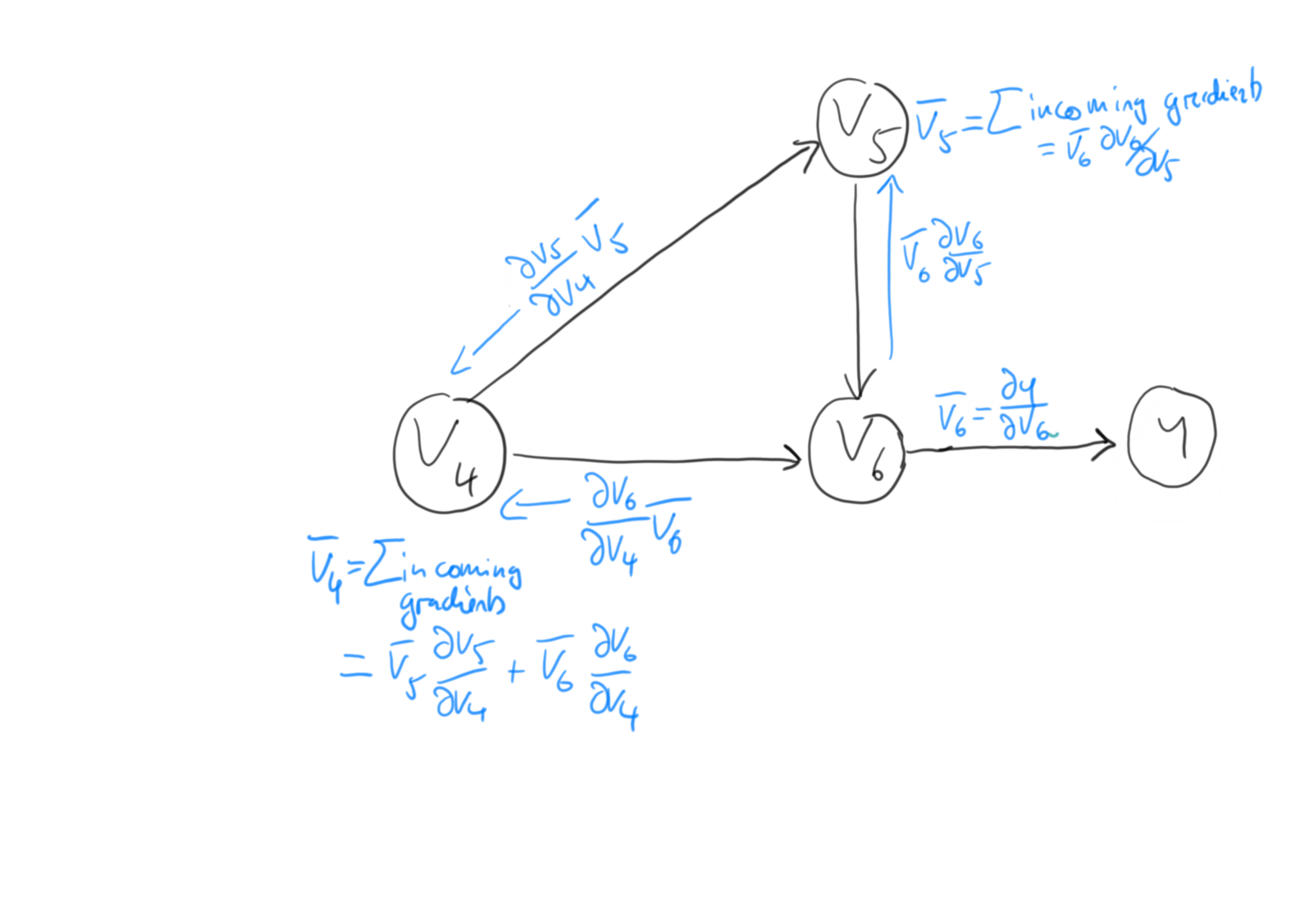
We see that there are two gradients incoming to the $v_4$ node: $\bar{v}_5 \partial v_5 / \partial v_4$ and $\bar{v}_6 \partial v_6 / \partial v_4$. Assuming that $\bar{v}_6$ and $\bar{v}_5$ are already evaluated, we just need the partial derivatives $\partial v_5 / \partial v_4$ and $\partial v_6 / \partial v_4$ to find $\bar{v}_4$:

$$\begin{align} \bar{v}_4 = \bar{v}_5 \frac{\partial v_5}{\partial v_4} + \bar{v}_6 \frac{\partial v_6}{\partial v_4} = \bar{v}_5 (-1) + \bar{v}_6 v_5. \end{align}$$

And indeed, we have recovered the same rule as when applying the chain rule. When we continue to calculate derivatives $\bar{v}_i$, we see that this notation becomes very handy. For example, using the chain rule we have

$$\begin{align} \bar{v}_3 = \frac{\partial y}{v_3} = \bar{v}_6 \frac{\partial v_6(v_5(v_4(v_1,v_3), v_4(v_3, v_1)))}{\partial v_3} \end{align}$$

where we again need to use the product rule. Using the bar-notation however, the derivative becomes trivial

$$\begin{align} \bar{v}_3 = \bar{v}_4 \frac{\partial v_4}{v_3} = \bar{v}_4 v_1, \end{align}$$

given that both $\bar{v}_4$ and $v_1$ have been evaluated. But in typical reverse-mode use this is the case, as we have completed one forward pass through the graph and we have traversed the barred values from right to left.

For completeness sake, let’s calculate the Reverse-mode AD evaluation trace as we did for the forward mode.

Reverse-mode AD evaluation trace
$v_{-1} = x_1 = 1.0$
$v_0 = x_2 = 1.1$
$v_1 = v_0 v_{-1} = (1.1) (1.0) = 1.1$
$v_2 = exp(v_1) = 3.004$
$v_3 = cos(v_0) = 0.4536$
$v_4 = v_1 v_3 = 0.4990$
$v_5 = v_2 - v_4 = (3.004) - (0.4990) = 2.5052$
$v_6 = v_4 v_5 = (0.4990) (2.5052) = 1.2500$
$\bar{v}_6 = \frac{\partial y}{\partial v_6} = 1$
$\bar{v}_5 = \frac{\partial y}{\partial v_5} = \bar{v}_6 v_4 = (1) (0.4990) = 0.4990$
$\bar{v}_4 = \frac{\partial y}{\partial v_4} = \bar{v}_6 \frac{\partial v_6}{\partial v_4} + \bar{v}_5 \frac{\partial v_5}{v_4} = \bar{v}_6 v_5 + \bar{v}_5 (-1) = (1)(2.5052) + (0.4990)(-1) = 2.006$
$\bar{v}_3 = \frac{\partial y}{v_3} = \bar{v}_4 \frac{\partial v_4}{\partial v_3} = \bar{v}_4 v_1 = (2.006) * (1.1) = 2.2069$
$\bar{v}_2 = \bar{v}_5 \frac{\partial v_5}{\partial v_2} = \bar{v}_5 (1) = 0.4990$
$\bar{v}_1 = \bar{v}_2 \frac{\partial v_2}{\partial v_1} + \bar{v}_4 \frac{\partial v_4}{\partial v_1} = \bar{v}_2 \exp(v_1) + \bar{v}_4 v_3 = (0.4990) (3.004) + (2.006)(0.4536) = 2.4090$
$\bar{v}_0 = \bar{v}_3 \frac{\partial v_3}{\partial v_0} + \bar{v}_1 \frac{\partial v_1}{\partial v_0} = \bar{v}_3 (- \sin v_0) + \bar{v}_1 v_{-1} = (2.2069) (-0.8912) + (2.4090)(1) = 4.3758$
$\bar{v}_{-1} = \bar{v}_1 \frac{\partial v_1}{\partial v_{-1}} = \bar{v}_1 v_0 = (2.4090) * (1.1) = 2.6500$

As a first step, we are evaluating all the un-barred quantities $v_i$ before we begin the backward pass, where we evaluate all the $\bar{v}_i$. We also see that we need the values of the child nodes to calculate the barred values. For example, to calculate $\bar{v}_3$ we need the value of $v_1$, which is a child-node of $v_4$, when evaluating the partial derivative $\partial v_4 / \partial v_1$.

We also see that this procedure would allow us to calculate the derivatives $\partial y / \partial v_i$ for an arbitrary number of $v_i$s in a single reverse pass. This is the exactly the behaviour that makes reverse-mode automatic differentiation so powerful in context of gradient-based optimization. In that situation we want to take the derivative of a scalar loss function with respect to a possible large amount of parameters.

Reverse-mode AD in higher dimensions: Jacobian-Vector products

We are often working in higher dimensional spaces, hidden layers in multilayer perceptrons for example can have hundreds or even thousands of features. It is therefore instructive to take a look how reverse-mode AD works in this setting. For this we are looking at a new example:

$$\begin{align} x \in \mathbb{R}^{n} \quad f: \mathbb{R}^{n} \rightarrow \mathbb{R}^{m} \quad g: \mathbb{R}^{m} \rightarrow \mathbb{R}^{l} \quad u \in \mathbb{R}^{m} \quad y \in \mathbb{R}^{l} \\ u = f(x) \quad y = g(u) = g(f(x)) \end{align}$$

The computational graph for the program $y = g(f(x))$ is just

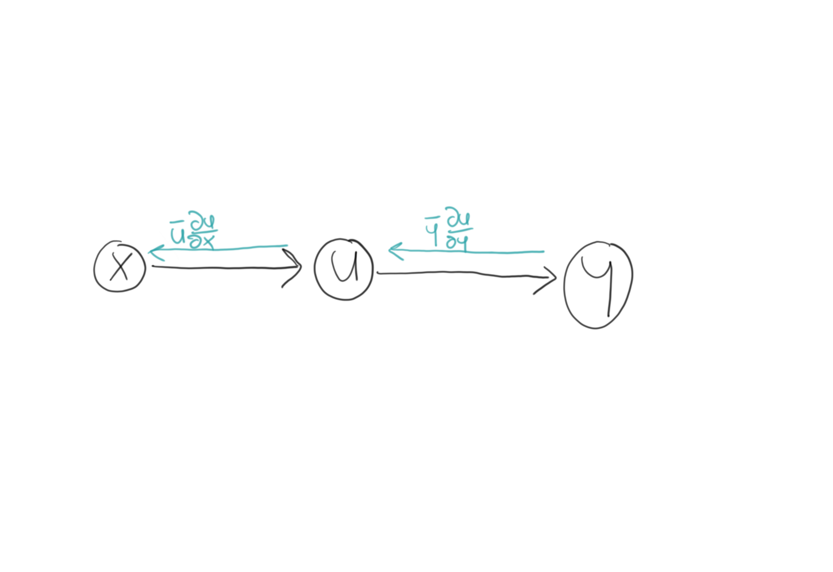
Now the formulas for the higher-dimensional case arise naturally from the ones derived in the previous section. Since we are discussing reverse mode, we start at the right. The bar quantities for each element of the first hidden layer is given by:

$$\begin{align} \bar{u}_j & = \sum_{i} \bar{y}_i \frac{\partial y_i}{\partial u_j} \\ \end{align}$$

Using vector notation, this equation can be written as

$$\begin{align} \left[ \bar{y}_1 \ldots \bar{y}_l \right] \left[ \begin{matrix} \frac{\partial y_1}{\partial u_1} & \ldots & \frac{\partial y_1}{\partial u_m} \\ \vdots & \ddots & \vdots \\ \frac{\partial y_l}{\partial u_1} & \ldots & \frac{\partial y_l}{\partial u_m} \end{matrix} \right] & = \left[ \bar{u}_1 \ldots \bar{u}_m \right] \end{align}$$

Now $\bar{f}$ is the vector that we get as an output from that calculation and will be propagated left-wards. We obtain it by calculating a vector-jacobian product. In practice, one usually does not calculate the jacobian matrix, but it is more efficient to calculate the vjp directly.

Moving leftwards to the graph, we use the same procedure to calculate $\bar{x}$:

$$\begin{align} \left[ \bar{u}_1 \ldots \bar{u}_n \right] \left[ \begin{matrix} \frac{\partial u_1}{\partial x_1} & \ldots & \frac{\partial u_1}{\partial x_n} \\ \vdots & \ddots & \vdots \\ \frac{\partial u_m}{\partial x_1} & \ldots & \frac{\partial u_m}{\partial x_n} \end{matrix} \right] & = \left[ \bar{x}_1 \ldots \bar{x}_n \right] \end{align}$$

Combining these results we find

$$\begin{align} \bar{x} = \bar{y} \left[ \left\{ \frac{\partial y_i}{\partial u_j} \right\}_{i,j} \right] \left[ \left\{ \frac{\partial u_i}{\partial x_j} \right\}_{r,s} \right]. \end{align}$$

This equation is evaluated left-to-right, so that it requires to calculate only vector-matrix products.

As a final note, these vector-jacobian products are often called pullbacks in the context of automatic differentiation software. A notation used for them is

$$\begin{align} \bar{u} = \sum_{i} \bar{y}_i \frac{\partial y_i}{\partial u} = \mathcal{B}^{u}_{f}(\bar{y}). \end{align}$$

Let’s unpack the expression $\mathcal{B}^{u}_{f}(\bar{y})$. The upper index denotes simply that the pullback is a function of $u$, since it needs the values from the forward-pass at the node to be evaluated. The lower index $f$ denotes that it depends on the mapping $f$, since this is the mapping from $x$ to $u: f(x) = u$. Finally, the argument $\bar{y}$ denotes that the pullback needs the incoming gradient from the right.

In practice, automatic differentiation software uses the chain rule to split the computational graph of a program into finer units until it can identify a pullback for a segment of the computational graph. In some cases this may be the desired way to work and in some cases, a user-defined backpropagation rule may be desireable.

Summary

We have introduced reverse-mode automatic differentiation. By starting with a gradient at the end of the computational graph, this mode allows to quickly calculate the sensitivity of an output with respect to an arbitrary large amount of intermediate values. To aid the necessary computations for this, the bar-notation has been introduced. Finally, we motivated that reverse-mode AD only needs to calculate vector-jacobian products and introduced the notation of pullback as the primitive object of reverse-mode AD. And finally, please check out the references below which I used for this blog-post.

References

[1] C. Rackauckas 18.337J/6.338J: Parallel Computing and Scientific Machine Learning

[2] S. Radcliffe Autodiff in python

[3] R. Grosse Lecture notes CSC321

[4] A. Griewank, A. Walther - Evaluating Derivatives - SIAM(2008)