Automatic differentiation - Forward Mode
Automatic differentiation allows one to take derivatives of computer programs which calculate numerical values. The name refers to a set of techniques that produce a transformed computer program which in turn calculates various derivatives of these values.
To see why this is extremely useful, consider a traditional data fitting problem. We have a model \(f_\theta: \mathbb{R}^m \rightarrow \mathbb{R}^n\), where \(\theta\) are the model parameters and observations \(y_i \in \mathbb{R}^n\) taken at \(x_i \in \mathbb{R}^{m}\). To fit the model on the data we can use a loss function, for example the mean-squared error
\[\begin{align} \mathcal{L} = \sum_{i} \left( f_\theta(x_i) - y_i \right)^2 \end{align}\]and tune the parameters \(\theta\) in order to minimize \(\mathcal{L}\). This process is also called learning or solving an inverse problem.
A common method to tune the parameters \(\theta\) is gradient descent. Given a learning rate \(\eta\) one iterates
\[\theta \leftarrow \theta - \eta \frac{\partial \mathcal{L}}{\partial \theta}\]until \(\mathcal{L}\) is approximately at a local minimum. Applying the chain rule, we can expand the derivative as
\[\frac{\partial \mathcal{L}}{\partial \theta} = \sum_i 2 \left( f_\theta(x_i) - y_i \right) \frac{\partial f_\theta(x_i)}{\partial \theta}.\]To perform the optization procedure we need to calculate the derivatives described by the last term in the equation above. This is where automatic differentiation comes into play.
A Toy Example
To better understand what automatic differentiation does and how it works let us consider the toy example
\[f(x_1, x_2) = x_1 x_2 \cos(x_2) \left[ \exp(x_1 x_2) - 1 \right] = y.\]In the following we will investigate how to calculate the derivative of \(f\) with respect to its inputs \(x_1\) and \(x_2\). In the context of the previous section, we can think of \(x_1\) as a parameter \(\theta\) that we wish to tone. While the method we present here is as simple as possible - real-world examples of tunable models often have thousands, millions, or even billions of parameters - it serves well to introduce the fundamental way in which automatic differentiation works. For the work below we are following [1] closely.
This mathematical formula for \(f\) can be decomposed into a succession of elementary functions, like \(+\), \(\sin\), \(\exp\), \(*\). That is, we can define intermediate variables like \(v_1(a,b) = a \cdot b\), \(v_2(a) = \cos a\) etc, which are only defined once. Each of these variables is also initialized by applying a simple expression to previous variables. Applying this procedure to our toy example gives us the following sequence:
| A simple program broken up into intermediate values |
|---|
| \(v_{-1} = x_1\) |
| \(v_{0} = x_2\) |
| \(v_{1} = v_{-1} \cdot v_{0}\) |
| \(v_{2} = \exp v_1\) |
| \(v_{3} = \cos v_0\) |
| \(v_{4} = v_1 \cdot v_3\) |
| \(v_{5} = v_2 - v_4\) |
| \(v_6 = v_4 v_5\) |
| \(y = v_6\) |
We now define the so-called Tangential Derivative \(\dot{v_i} = \partial v_i / \partial x_1\). For the tangential derivative, we are fixing the denominator to \(x_1\) so that it describes the sensitivity of the functions output with respect to the given input. Let us calculate this derivative for the v’s now:
\[\begin{align} \dot{v}_1 & = \frac{\partial v_1}{\partial x_1} = v_0 \frac{\partial v_{-1}}{\partial v_{-1}} = v_0 \\ \dot{v}_2 & = \frac{\partial v_2}{\partial v_1} \dot{v}_1 = v_0 \exp v_1\\ \dot{v}_3 & = \frac{\partial v_3}{\partial v_0} \dot{v}_0 = 0 \\ \dot{v}_4 & = \frac{\partial v_4}{\partial v_1} \dot{v}_1 + \frac{\partial v_4}{\partial v_3} \dot{v}_3 = v_3 v_0 \\ \dot{v}_5 & = \frac{\partial v_5}{\partial v_2} \dot{v}_2 + \frac{\partial v_5}{\partial v_4} \dot{v}_4 = \dot{v}_2 - \dot{v}_4 \\ \dot{v}_6 & = \frac{\partial v_6}{\partial v_5} \dot{v}_5 + \frac{\partial v_6}{\partial v_4} \dot{v}_4 = \dot{v}_5 v_4 + \dot{v}_4 v_5 \\ \end{align}\]Note that we have to use \(\dot{v}_{-1} = 1\) and \(\dot{v}_{0} = 0\) in order to calculate \(v\dot{v}_1\). That is, the seed determines which part of the sum is non-zero. From the expressions above we can alos see that we will need to evaluate the derivatives starting at \(v_1\). That is, we begin at the start of the function, calculate simple derivatives and push this calculation through. Therefore this is also called forward mode automatic differentiation.
In practice, forward mode AD is often implemented by operator overloading. An implementation would need seed an initial derivative \(x_i = 1\) and then calculate the program and the derivatives simultaneously. This approach works for our toy example as we see from the evaluation trace shown below:
| Forward-mode AD evaluation trace | |
|---|---|
| \(v_{-1} = x_1 = 1.0\) | \(\dot{v}_{-1} = 1.0\) |
| \(v_{0} = x_2 = 1.1\) | \(\dot{v}_{0} = 0.0\) |
| \(v_1 = v_0 v_{-1} = (1.1) (1.0) = 1.1\) | \(\dot{v}_{1} = v_{0} = (1.1)\) |
| \(v_{4} = v_1 v_3 = (1.1) (0.4536) = 0.4990\) | \(\dot{v}_4 = v_3 \dot{v}_1 = (0.4536) * (1.1) = 0.499\) |
| \(v_{5} = v_2 - v_4 = (3.004) - (0.4990) = 2.5052\) | \(\dot{v}_5 = \dot{v}_2 - \dot{v}_4 = 3.305 - 0.499 = 2.851\) |
| \(v_6 = v_4 v_5 = (0.4990) (2.7180) = 1.2500\) | \(\dot{v}_6 = v_4 \dot{v}_5 + \dot{v}_4 v_5 = (0.499) (2.851) + (0.499) (2.505) = 2.650\) |
It is illustrative to visualize how the values and derivatives are propagated in the computational graph.
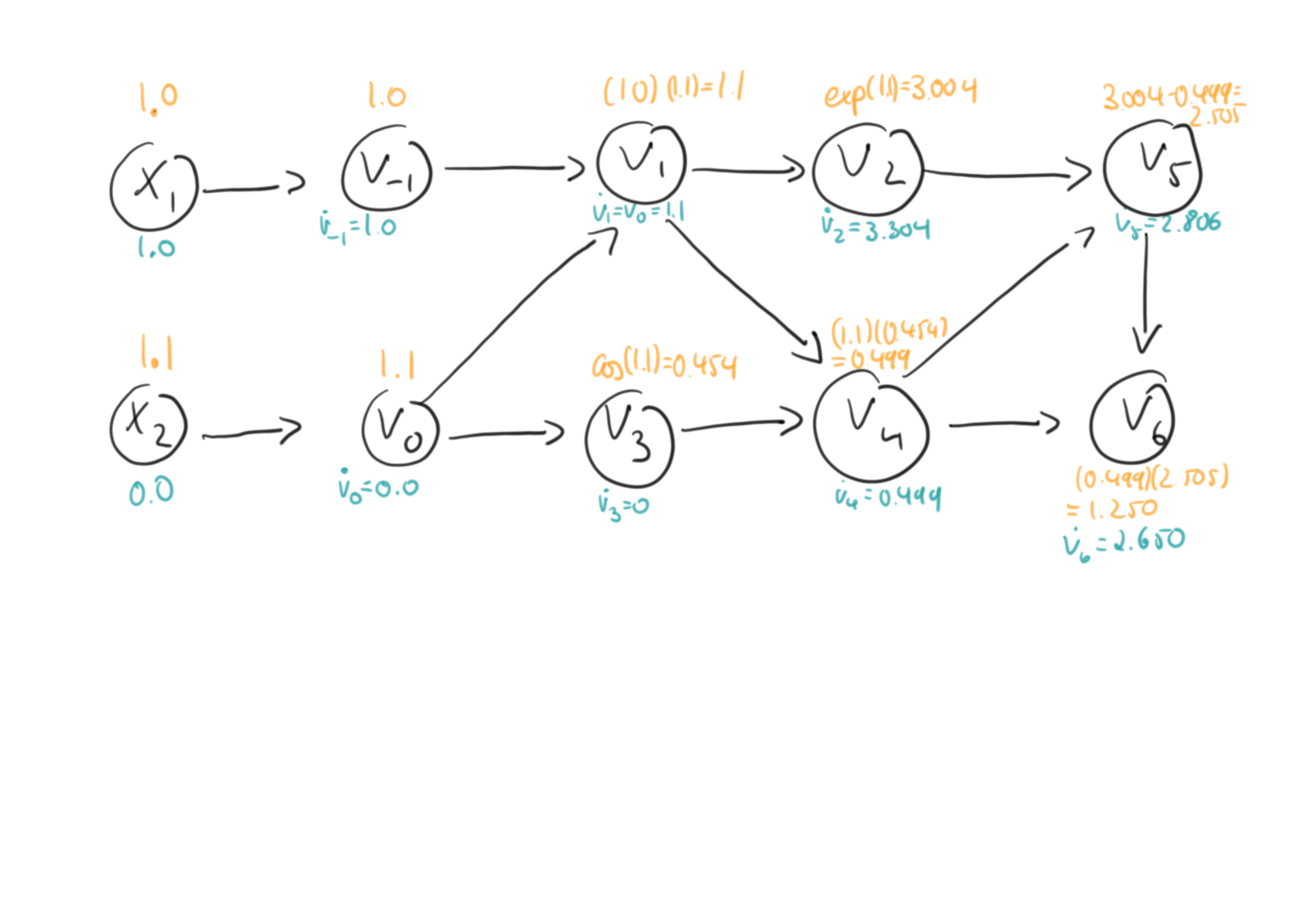
Here the intermediate values are shown in yellow and the gradient values are shown in turquoise. Note that both, values and derivatives are propagated together from the left, the input, to the output on the right. The implication of this is that forward-mode autodiff can calculate the sensitivities of all outputs y with respect to one input x in a multidimensional setting.
Summary
Automatic differentiation is a set of tools that allows to calculate the derivatives of computer programs that return numerical values. Here we looked at the so-called forward mode of automatic differentiation. It works by de-composing a program into simple functions for which we know the derivative. We can initialize a program and set the input variable for which we want to know the output’s derivatives for. Then we can calculate the function value and the derivative of the output with respect to the chosen value in one sweep.
This works well for situations where we have a small number of inputs and a large number of outputs. But in data-fitting problems we often end up with the reverse situation: We have a large number of outputs and few, or maybe only a single output. In these situations one may want to use reverse-mode automatic differentiation.
References
[1] A. Griewank, A. Walther - Evaluating Derivatives - SIAM(2008)