Backpropagating through QR decomposition
One of the most useful decompositions of Linear Algebra is the QR decomposition. This decomposition is particularly important when we are interested in the vector space spanned by the columns of a matrix A. Formally, we write the QR decomposition of \(A \in \mathbb{R}^{m \times n}\), where m ≥ n, as
\[\begin{align} A = QR = \left[ \begin{array}{c|c|c|c} & & & \\ q_1 & q_2 & \cdots & q_n \\ & & & \end{array} \right] % \left[ \begin{array}{cccc} r_{1,1} & r_{1,2} & \cdots & r_{1,n} \\ 0 & r_{2,2} & \cdots & r_{2,n} \\ 0 & 0 & \ddots & \vdots \\ 0 & \cdots & & r_{n,n} \end{array} \right]. \end{align}\]Where Q is an orthogonal m-by-n matrix, i.e. the columns of Q are orthogonal \(q_{i} \cdot q_{j} = \delta_{i,j}\). R is a square n-by-n matrix. Using the decomposition, we can reconstruct the columns of A as
\[\begin{align} a_1 & = r_{1,1} q_1 \\ a_2 & = r_{1,2} q_1 + r{2,2} q_2 \\ & \cdots \\ a_n & = \sum_{j=1}^{n} r_{j,n} q_j. \end{align}\]Internally, Julia treats QR-factorized matrices through a packed format [1]. This format does not store the matrices Q and R explicitly, but using a packed format. All matrix algebra and arithmetic is implemented through methods that expect the packed format as input. And the QR decomposition itself is calling the LAPACK method geqrt which returns just this packed format.
A computational graph where one may want to backpropagate through a QR factorization
may look similar to this one:
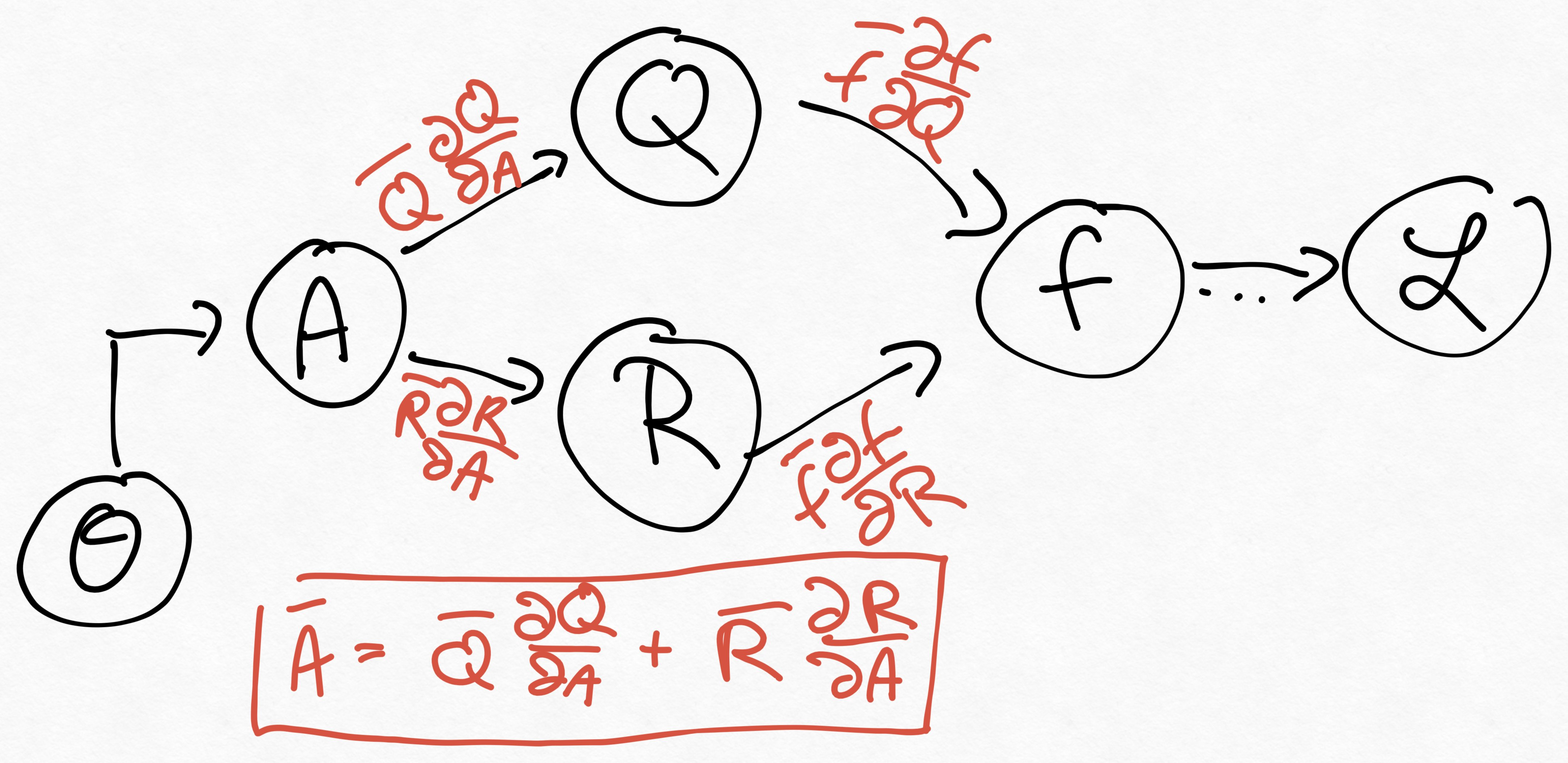
While the incoming gradients, \(\bar{f} \partial f / \partial Q\) and \(\bar{f} \partial f / \partial R\) depend on \(f\), the gradients for the QR decomposition \(\bar{Q} \partial Q / \partial A\) and \(\bar{R} \partial R / \partial A\) are defined through the QR factorization. While these can be in principle computed through an automatic differentiation framework, it can be beneficial to implement a pullback. For one, this saves compilation time before first execution. An additional benefit is less memory use, as the gradients will be propagated through fewer functions. A pullback for the QR factorization may thus also aid numerical stability, as fewer accumulations and propagations are performed.
Formulas for the pullback of the QR factorization are given in [2], [3] and [4]. Pytorch for example implements the method described in [3], see here.
In this blog post, we implement the pullback for the QR factorization in Julia. Specifically, we implement a so-called rrule for ChainRules.jl. While you are here, please take a moment and read the documentation of this package. It is very well written and helped me tremendously to understand how automatic differentiation works and is implemented n Julia. Also, if you want to skip ahead, here is my example implementation of the QR pullback for ChainRules.
Now, let’s take a look at the code and how to implement a custom rrule. The first thing we need to look at is the definition of the QR struct
struct QR{T,S<:AbstractMatrix{T}} <: Factorization{T}
    factors::S
    τ::Vector{T}

    function QR{T,S}(factors, τ) where {T,S<:AbstractMatrix{T}}
        require_one_based_indexing(factors)
        new{T,S}(factors, τ)
    end
end
There are two fields in the structure, factors and τ. The matrices Q and R are returned through an accompanying getproperty function:
function getproperty(F::QR, d::Symbol)
    m, n = size(F)
    if d === :R
        return triu!(getfield(F, :factors)[1:min(m,n), 1:n])
    elseif d === :Q
        return QRPackedQ(getfield(F, :factors), F.τ)
    else
        getfield(F, d)
    end
end
For the QR pullback we first need to implement a pullback for the getproperty function. The pullback for this function only propagates incoming gradients backwards. Incoming gradients are described using a Tangent. This struct can only have fields that are present in the parameter type, in our case LinearAlgebra.QRCompactWY. This struct has fields factors and τ as discussed above. Now the incoming gradients would be \(\bar{Q}\) and \(\bar{R}\). Thus the pullback needs to map between these two. Thus the pullback can be implemented like this:
function ChainRulesCore.rrule(::typeof(getproperty), F::LinearAlgebra.QRCompactWY, d::Symbol)
    function getproperty_qr_pullback(Ȳ)
        ∂factors = if d === :Q
            Ȳ
        else
            nothing
        end

        ∂T = if d === :R
            Ȳ
        else
            nothing
        end

        ∂F = Tangent{LinearAlgebra.QRCompactWY}(; factors=∂factors, T=∂T)
        return (NoTangent(), ∂F)
    end

    return getproperty(F, d), getproperty_qr_pullback
end
Notice the call signature of the rrule. The first argument is always
::typeof(functionname), where functionname is the name of the function that
we want a custom rrule for. Following this argument are the actual arguments
that one normally passes to functionname.
Finally we need to implement the pullback that actually performs the relevant calculations. The typical way of implementing custom pullbacks with ChainRules is write a function that calculates that returns a tuple containing the result of the forward pass, as well as the pullback \(\mathcal{B}^{x}_{f}(\bar{y})\). Doing it this way allows the pullback to re-use results from the forward pass. In other words, by defining the pullback as a function in the forward pass allows to easily use cached results. There is more discussion on the reason behind this design choice in the ChainRules documentation.
Returning to the pullback for the QR factorization, here is a possible implementation:
function ChainRules.rrule(::typeof(qr), A::AbstractMatrix{T}) where {T}
    QR = qr(A)
    m, n = size(A)
    function qr_pullback(Ȳ::Tangent)
        function qr_pullback_square_deep(Q̄, R̄, A, Q, R)
            M = R̄*R' - Q'*Q̄
            # M <- copyltu(M)
            M = triu(M) + transpose(triu(M,1))
            Ā = (Q̄ + Q * M) / R'
        end
        Q̄ = Ȳ.factors
        R̄ = Ȳ.T
        Q = QR.Q
        R = QR.R
        if m ≥ n
            Q̄ = Q̄ isa ChainRules.AbstractZero ? Q̄ : @view Q̄[:, axes(Q, 2)]
            Ā = qr_pullback_square_deep(Q̄, R̄, A, Q, R)
        else
            # partition A = [X | Y]
            # X = A[1:m, 1:m]
            Y = A[1:m, m + 1:end]

            # partition R = [U | V], and we don't need V
            U = R[1:m, 1:m]
            if R̄ isa ChainRules.AbstractZero
                V̄ = zeros(size(Y))
                Q̄_prime = zeros(size(Q))
                Ū = R̄
            else
                # partition R̄ = [Ū | V̄]
                Ū = R̄[1:m, 1:m]
                V̄ = R̄[1:m, m + 1:end]
                Q̄_prime = Y * V̄'
            end

            Q̄_prime = Q̄ isa ChainRules.AbstractZero ? Q̄_prime : Q̄_prime + Q̄

            X̄ = qr_pullback_square_deep(Q̄_prime, Ū, A, Q, U)
            Ȳ = Q * V̄
            # partition Ā = [X̄ | Ȳ]
            Ā = [X̄ Ȳ]
        end
        return (NoTangent(), Ā)
    end
    return QR, qr_pullback
end
The part of the rrule that calculates the foward pass just calculates the QR decomposition and returns the result of that. The pullback consumes the incoming gradients, \(\bar{R}\) and \(\bar{Q}\), which are stored as defined in the pullback for getproperty. The actual calculation for the case where the dimensions of the matrix A are equal, m=n, and the case where A is tall and skinny, m>n are different. But they can re-use some code. That is what the local function qr_pullback_square_deep does. The rest is mostly matrix slicing and the occasional matrix product. The implementation is borrows strongly from pytorch’s autograd implementation.
Finally, I need to verify that my implemenation calculates correct results. For this, I define two small test functions which each work on exactly one output of the QR factorization, either the matrix Q or the matrix R. Then I generate some random input and compare the gradient calculated through reverse-mode AD in Zygote to the gradient calculated by FiniteDifferences. If they are approximately equal, I take the result to be correct.
V1 = rand(Float32, (4, 4));

function f1(V) where T
    Q, _ = qr(V)
    return sum(Q)
end

function f2(V) where T
    _, R = qr(V)
    return sum(R)
end


res1_V1_ad = Zygote.gradient(f1, V1)
res1_V1_fd = FiniteDifferences.grad(central_fdm(5,1), f1, V1)
@assert res1_V1_ad[1] ≈ res1_V1_fd[1]
[1] Schreiber et al. A Storage-Efficient WY Representation for Products of Householder Transformations
[2] HJ Liao, JG Liu et al. Differentiable Programming Tensor Networks
[3] M. Seeger, A. Hetzel et al. Auto-Differenting Linear Algebra
[4] Walter and Lehman Walter and Lehmann, 2018, Algorithmic Differentiation of Linear Algebra Functions with Application in Optimum Experimental Design