This post is a follow-up from the last one. But now we are focusing on solving a non-linear system of the form

\[F(x) = 0\]

using a quasi-Newton method. You find the definition on Wikipedia. Basically it is Newton’s method but you replace the Jacobian with an approximation. In this blog post we are considering a simple two-dimensional system. Using Newton’s method for this example is trivial and leads to a converged solution after only two or three steps, since it converges quadratically. A quasi-Newton method on the other hand converges only linearly. And we aim to improve on that convergence behaviour by using a machine-learned preconditioner. Now, preconditioners are usually used to accelerate convergence of linear solvers, like GMRES. And I don’t claim that they are generally useful for non-linear systems. So we do it just to see if this works in principle.

Quasi-Newton iteration

We consider the simple two-dimensional system

\[\begin{align} F_1(x_1, x_2) = x_1 + \alpha x_1 x_2 - s_1 & = 0 \\ F_2(x_1, x_2) = \beta x_1 x_2 + x_2 - s_2 & = 0 \end{align}\]

where $\alpha$ and $\beta$ are of the order 0.01 and the source terms are $s_{1,2} \sim \mathcal{N}(1, 10^{-2})$. Picking the source terms from a Normal distribution allows us to consider a large number of instances of this problem. Later we will use this to generate training and test sets.

Newton’s method can be used to find the root of $F(x)$. Starting out at an initial guess $x_0$, it updates the guess by guiding it along its gradient: $F(x_0 + \delta x) \approx F(x_0) + J(x) \delta x \approx 0$. Here $J^{-1}(x)$ is the inverse of an approximation on the Jacobian Matrix whose entries are is defined as $(J(x))_{ij} = \partial F_i / \partial x_j$. Solving for $\delta x$ gives the update $\delta x = J^{-1}(x) F(x)$. Now the Jacobian matrix of the system can be easily calculated. For the quasi-Newton method we consider the approximation

\[\widetilde{J}(x) = \begin{pmatrix} 1 + \alpha x_2 & 1 \\ 1 & 1 + \beta x_1 \end{pmatrix}\]

where the off-diagonal elements of the original Jacobian have been modified as $\partial F_1 / \partial x_2 = \alpha x_1 \approx 1$ and $\partial F_2 / \partial x_1 = \beta x_2 \approx 1$.

A quasi-Newton aims to find the root of $F(x)=0$ using the same iteration scheme but using an approximation to the Jacobian instead $\begin{align} x_{k+1} & = x_k - \widetilde{J}^{-1}(x) f(x). \end{align}$

If you use the true Jacobian you have Newton’s method and the rate of convergence is quadratic. If you don’t, you have a quasi-newton method and the rate of convergence is linear. How can we accelerate convergence in this case?

To accelerate convergence, we can use a Preconditioner $P^{-1}$. This is a invertible matrix that we squeeze into the update by inserting a one:

\[\begin{align} J(x_k) \delta x_k &= -F(x_k) \Leftrightarrow \\ \left( J(x_k)P^{-1} \right) \left( P \delta x_k \right) &= -F(x_k) \end{align}\]

The update from $x_k \rightarrow x_{k+1}$ then needs to calculated in two steps.

Calculate $\delta w = \left( \widetilde{J} \right)^{-1} P^{-1} \left(F(x_k) \right)$
Calculate $\delta x_{k} = P^{-1} \delta w$.
Update $x_{k+1} = x_{k} + \delta_x$.

That is, we apply $P^{-1}$ twice. A closed form of $P$ is not required. Next we will see how to implement $P^{-1}$ as a neural network and how to train it using differentiable code.

Neural-Network preconditioner

We parameterize the preconditioner with a Multilayer perceptron as $P^{-1}_{\theta}: \mathbb{R}^{m} \rightarrow \mathbb{R}^2$:

using Flux
dim = 2
Pinv = Chain(Dense(2*dim + 2, 50, celu), Dense(50, 50, celu), Dense(50, dim))

Here we allow for $m > 2$ to pass additional inputs to the Network. We are also using CeLU activation functions to avoid having a non-differentiable point at $x=0$ and we are choosing a simple 3-layer feed-forward architecture to start out with.

While this gives us a parameterization we now have to find out how to train the network. The task of the preconditioner is to minimize the residual after $n_\mathrm{i}$ iterations of Newtons method. The following loss function tells us how well $P^{-1}$ is doing over a number of examples $F(x) = 0$, where the RHS terms $s_1, s_2 \sim \mathcal{N}\left(2, 0.01\right)$.

sqnorm(x) = sum(abs2, x) 


function loss2(batch)
# batch is a 2d-array. dim1: index within batch. dim2: indices the batch
    # Loss of the current sample. Defined as the norm of f(x) after nᵢ Newton iterations
    loss_local = 0.0
    # Batch-size
    batch_size = size(batch)[2]
    # Iterate over source vectors in the current mini-batch
    for sidx in 1:batch_size
        # Grab the current source terms 
        s = batch[:, sidx]
        # Define a RHS
        function f(x) 
            F = Zygote.Buffer(zeros(dim))
            F[1] = x[1] + α*x[1]*x[2] - s[1]
            F[2] = β * x[1] * x[2] + x[2] - s[2]
            return copy(F)
        end

        # run num_steps of Newton iteration for the current RHS
        sol = picard(x, x0, Pinv, s, 1)
        loss_local += norm(f(sol))
    end

    return log(loss_local) / batch_size
end

One has to be careful in evaluating the preconditioner within calls to the Picard iteration. After each iteration, the input $f(x)$ will decrease by an order of magnitude. Neural Networks work best of the input is of order one on the other hand. Thus we need to find a way to provide input of order one to $P^{-1}$ at each iteration. In the routine below the input is

$f(x) / \vert f(x) \vert_{2}$ - Input $f(x)$, scaled to its L² norm
$s$ - The source terms in $F(x) = 0$.
$\log \vert f(x) \vert$ - Gives the order of magnitude of the input
$i$ - The current iteration

The first term represents the desired input, re-scaled to be order unity, and the logarithm $\log \vert f(x) \vert$ estimates the order of magnitude of this term. For example for $\vert f(x) \vert = 10^{-5} \rightarrow \log \vert f(x) \vert \approx -11.5$. I also pass the source term $s$ and the current Picard iteration $i$ into $P^{-1}$.

function picard(f, x, P⁻¹, s, num_steps)
# Run num_Steps of Newton iteration
# P⁻¹: Preconditioner
# s: source terms in F(x) + s = 0

    for i = 1:num_steps
        # P⁻¹ receives the following inputs
        # f(x) / norm(f(x)) : Scaled input
        # s                 : source term
        # log(norm(f(x)))   : Order of magnitude of f(x)
        # i                 : Iteration number I
        δw = pinv(J(x)) * P⁻¹(vcat(f(x) / norm(f(x)), s, log(norm(f(x))), i))
        δx = P⁻¹(vcat(δw / norm(δw), s, log(norm(δw)), i))
        x = x - δx
    end
    return x
end

I am generating 100 training samples which I divide into 10 mini-batches for training. Similarly, the test-set is 100 examples. Here I don’t use a validation set but instead only consider the loss on the training set. While training I am monitoring the loss on the training set. If it has not decreased for 5 epochs, I’m halfing the learning rate.

In order to optimize the neural network as to give a smaller residual after one iteration one needs to calculate the gradients of the loss with respect to the parameters of the neural network. Zygote allows us to do this using only a single call to gradient:

   
# Start training loop
loss_vec = zeros(num_epochs)
η_vec = zeros(num_epochs)
# Counts how many steps we haven't improved the loss function.
stall_thresh = 5

for epoch in 1:num_epochs
    # Randomly shuffly the training examples
    batch_idx = shuffle(1:num_train)
    for batch in 1:num_batch
        # Get random indices for the current batch
        this_batch = batch_idx[(batch - 1) * batch_size + 1:batch * batch_size]
        grads = Flux.gradient(Flux.params(P⁻¹)) do 
            l = loss2(source_train[:, this_batch])
        end
        for p in Flux.params(P⁻¹)
            Flux.Optimise.update!(p, -η * grads[p])
        end
        Zygote.ignore() do 
            loss_vec[epoch] = loss2(source_train[:, this_batch])
            η_vec[epoch] = η
            if mod(epoch, 10) == 0
                println("Epoch $(epoch) loss $(loss_vec[epoch])  η $(η)")
            end
        end
    end

    if (epoch > stall_thresh) && (loss_vec[epoch] > mean(loss_vec[epoch - stall_thresh:epoch]))
        global η *= 0.5
        println("    new η = $(η)   ")
    end
    if η < 1e-10
        break 
    end
end

Training the preconditioner is a bit tricky. I had to play quiet a bit with the layout of the network, the learning rate, and the batch size to get useful results. One setup that works is

x0 = [1.9; 2.2]
α = 0.03
β = -0.07

Pinv = Chain(Dense(2*dim + 2, 100, celu), Dense(100, 200, celu), Dense(200, 100, celu), Dense(100, dim))

num_train = 100
num_epochs = 100
num_batch = 10
num_test = 100

Let’s look at the loss on the training set:

Training loss

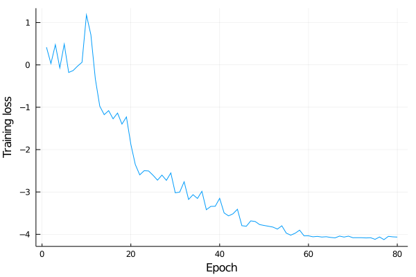
For the first few epochs, there is no significant training. But around epochs 10 and then 20, there are significant drops. After 20, training proceeds uniform and the loss function flattens out around epoch 60. Learning-rate scheduling is essential here, it is halfed around the steep drops. Finally we end up with an L² loss of about exp(-4)≈0.01 per sample.

We can evaluate the performance of the learned preconditioner by testing it on unseen examples:

or idx in 1:num_test
    # Load the source vector from the test set
    s = source_test[:, idx]
    # Define the non-linear system with the current source vector
    function f(x)
        F = zeros(dim)
        F[1] = x[1] + α * x[1] * x[2] - s[1]
        F[2] = β * x[1] * x[2] + x[2] - s[2]
        return F
    end

    # Run 1 iteration with ML preconditioner, store solution after 1 iteration in x1_ml
    x1_ml = newton(f, x0, P⁻¹, s, 1)
    # Run 1 iteration without preconditioner, store solution after 1 iteration in x1_no
    x1_no = newton_no(f, x0, 1)

    # Run 5 more newton iterations, starting at x1_ml
    vsteps_ml = map(n -> norm(f(newton_no(f, x1_ml, n))), 0:5)
    # Run 5 more newton iterations, starting at x1_no
    vsteps_no = map(n -> norm(f(newton_no(f, x1_no, n))), 0:5)
end

The first iteration is performed using the preconditioner, followed by 5 iterations without preconditioning. This is compared to the norm of the residuals in 6 iterations performed without preconditioner. The plot below shows the convergence history of 100 test samples. Green line show ML-preconditioned iterations, red lines show the iteration history without peconditioner.

Residual Loss

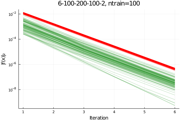
We find that the Neural Network can act as a preconditioner in the first iteration. The residual norm after one iteration shows large scatter, almost two orders of maagnitude. After one accelerated initial step, the iteration continues with linear rate of convergence for all test samples. That is at the same rate as the un-preconditioned samples, shown in red here.

In summary, yes, we can use a machine-learned preconditioner to accelerate Picard iteration to solve non-linear systems. It is a bit tricky to learn and I only showed how to do the first iteration. So there are still many details that have not been explored. I would also like to add that for the case here, Newton’s method is the way to go. It has a quadratic rate of convergence - much faster than the linear rate of Picard iteration. For the samples here, residuals are machine precision after about 3 to 4 iterations. But if that is not an option, using a Neural Network can accelerate your Picard iteration.