Machine-learned preconditioners - Part 1
What is a preconditioner?
A common task in scientific computing is to solve a system of linear equations
\[Ax = b\]with a matrix \(A \in \mathcal{R}^{d \times d}\) that gives the coefficients of the system, a right-hand-side vector \(b \in \mathcal{R}^{d}\), and a solution vector \(x \in \mathcal{R}^{d}\).
Instead of solving the linear problem directly, one often solves the preconditioned problem. We write this problem by inserting a one in the linear system and re-parenthesing:
\(\left( A P^{-1} \right) \left( P x \right) = b\) In this equation we have changed the coefficient matrix from \(A\) to \(A P^{-1}\) and the solution vector is now \(P x\) instead of \(x\). To retrieve the original vector, simply calculate \(x = P^{-1}y\). The matrix \(P^{-1}\) is called the preconditioner.
The dependence of \(P^{-1}\) on \(x\) is by choice. There is no deeper reason for why the preconditioner should depend on the initial guess for the iteraion. We choose to include this dependency here to foreshadow later applications, where such a dependency may be useful. In practice, this choice here is rather limiting. Since the matrix \(A_0 P^{-1}\) needs to be positive definite, and by construction only \(\widetilde{b}\) is positive definite, the method as constructed here is only valid for \(x \approx 0\).
The Gauss-Seidel method is an iterative method to find the solution of a linear system. Given an initial guess \(x_0\), update the entries of this vector following an iterative scheme and after some, or many, iterations, \(x_0\) solves the equation \(A x_0 = b\). Wikipedia has a nice and instructive page on this scheme.
A good preconditioner gives you a converged solution after fewer iterations. In other words, with a good preconditioner you are closer to the true solution of the linear system after N iterations than you are with a bad preconditioner. Choosing a good preconditioner depends on the problem at hand and can become a dark art. Let’s make it even more dark and train a neural network to be a preconditioner.
Modeling preconditioner as a neural network
As a first step, let’s model \(P^{-1}\) as a multi-layer perceptron (technically a single-layer):
\[P^{-1} = \sigma \left( W x + \widetilde{b} \right)\]with a weight matrix \(W \in \mathcal{R}^{d^2 \times d}\), a bias \(\widetilde{b} \in \mathcal{R}^{d^2}\), and a ReLU \(\sigma\). With \(x \in \mathcal{R}^{d}\) the matrix dimensions are chosen such that \(P^{-1}\) is of dimension \(d^2\). Simply reshape it to \(d \times d\) to have it act like a matrix.
Here I’m discussing a simple test case and am working with the Gauss-Seidel iterative solver. For real problem one would probably use a different iterative algorithm, but it serves as a proof-of-concept. Anyway, for Gauss-Seidel to work, the system coefficient matrix \(AP^{-1}\) needs to be positive-definite. How do we do this for our neural network? A simple hack is to consider only vectors whose entries are close to zero.
That way we get away with requiring only \(\widetilde{b}\) to be positive-definite. We get the last property by letting \(\widetilde{b} = b_0 b_0^{T}\) and sampling the entries of \(b_0\) as \(b_{ij} \sim \mathcal{N}(0, 1)\). In a similar fashion, we sample the entries of the weight-matrix \(W\) as \(w_{i,j} \sim \mathcal{N}(0,1)\).
How can we train a preconditioner
To make this preconditioner useful, the weights \(W\) and bias term \(b\) need to be optimized such that the residual after \(N\) iterations is as small as possible. And this needs to be true for all vectors from a training set. Using automatic differentiation, we can train \(W\) and \(b\) using gradient descent like this:
- Pick an initial guess \(x_0\) with \(x_{0,i} \sim \mathcal{N}(0, 0.01)\)
- Build the preconditioner \(P^{-1} = \sigma(W, x_0, \widetilde{b})\)
- Calculate 5 Gauss-Seidel steps. Let’s call the solution here \(y_5\).
- Un-apply the preconditioner: \(x_5 = P^{-1} y_5\)
- Calculate the distance to the true solution \(\mathcal{L} = \frac{1}{N} \sum_{i=1}^{N} \left( x_{\text{true}, i} - x_{5,i} \right)^2\)
- Calculate the gradients \(\nabla_{W} \mathcal{L}\) and \(\nabla_{B} \mathcal{L}\)
- Update the weight matrix and bias using gradient descent: \(W \leftarrow W - \alpha \nabla_{W} \mathcal{L}\) and \(b \leftarrow b - \alpha \nabla_{b} \mathcal{L}\). Here \(\alpha\) is the learning rate
The approach here is to directly back-propagate from the loss function \(\mathcal{L}\), through the numerical solver, to the parameters of the preconditioner \(W\) and \(b\). We are not working with an offline training and test-data set, but the data is taken directly from the numerical calculations. This way we directly capture the reaction of the numerical solver to updates proposed by gradient descent.
The derivatives \(\nabla_\theta \mathcal{L}\) can be calculate using automatic differentiation packges, such as Zygote.
Implementation
# Test differentiation through control flow

# Use a iterative conjugate solver with preconditioner

using Random
using Zygote
using LinearAlgebra
using Distributions
using NNlib
I copy-and-pasted the Gauss-Seidel code from wikipedia:
function gauss_seidel(A, b, x, niter)
    # This is from https://en.wikipedia.org/wiki/Gauss%E2%80%93Seidel_method
    x_int = Zygote.Buffer(x)
    x_int[:] = x[:]
    for n ∈ 1:niter
        for j ∈ 1:size(A, 1)
            x_int[j] = (b[j] - A[j, :]' * x_int[:] + A[j, j] * x_int[j]) / A[j, j]
        end
    end
    return copy(x_int)
end
The block below sets things up.
Random.seed!(1)
dim = 4

# Define a matrix
A0 = [10.0 -1.0 2.0 0.0; -1 11 -1 3; 2 -1 10 -1; 0 3 -1 8]
# Define the RHS
b0 = [6.0; 25.0; -11.0; 15.0]
# This is the true solution
x_true = [1.0, 2.0, -1.0, 1.0]

# Define the size of the training and test set
N_train = 100
N_test = 10

# Define an initial state. Draw this from a narrow distribution around zero
# We need to do this so that the preconditioner eigenvalues are positive
x0 = rand(Normal(0.0, 0.01), (N_train, dim))

# Define an MLP. This will later be our preconditioner
# The output should be a matrix and we work with 2dim as the size for the MLP
W = rand(dim*dim, dim)
# For Gauss-Seidel to work, the matrix A*P⁻¹ needs to be positive semi-definite.
bmat = rand(dim, dim)
# We know that any matrix A*A' is positive semi-definite
bvec = reshape(bmat * bmat', (dim * dim))
# Now Wx + bmat is positive semi-definite if x is very small
P(x, W, b) = NNlib.relu.(reshape(W*x .+ b, (dim, dim)))
# Positive-definite means positive Eigenvalues. We should check this.
@show eigvals(A0*P(x0[0,:], W, bvec))
This function will serve as our loss function. It evaluates the NN preconditioner and then runs some Gauss-Seidel iterations. Finally, the iterative solution approximation is transformed back by applying \(P^{-1}\).
function loss_fun(W, bmat, A0, b0, y0, niter=5)
    # W - Weight matrix for NN-preconditioner
    # bmat - Bias vector for NN preconditioner
    # A0: Linear system coefficient matrix
    # b0: RHS of linear system
    # y0 - initial guess for Linear system. Strictly, this is x0. But we call it the same
    # assuming that P⁻¹x0 = x0.
    # niter - Number of Gauss-Seidel iterations to perform

    loss = 0.0
    nsamples = size(y0)[1]

    for idx ∈ 1:nsamples:
        # Evaluate the preconditioner
        P⁻¹ = P(y0[idx, :], W, reshape(bmat * bmat', (dim * dim)))
        # Initial guess
        # Now we solve A(Px)⁻¹y = rhs for y with 3 Gauss-Seidel iterations
        y_sol = gauss_seidel(A0 * P⁻¹, b0, y0[idx, :], niter)
        # And reconstruct x
        x = P⁻¹ * y_sol
        loss += norm(x - x_true) / length(x)
    end

    return loss / nsamples
end
Now comes the fun part. Zygote calculates the partial derivatives of the loss function with respect to its input, in our case \(W\) and \(b\). Given the gradients, we can actually update \(W\) and \(b\).
# Number of epochs to train
num_epochs = 10
loss_arr = zeros(num_epochs)
# Store the Weight and bias matrix at each iteration
W_arr = zeros((size(W)..., num_epochs))
bmat_arr = zeros((size(bmat)..., num_epochs))
# Learning rate
α = 0.005

for epoch ∈ 1:num_epochs
    loss_arr[epoch], grad = Zygote.pullback(loss_fun, W, bmat, A0, b0, x0)
    res = grad(1.0)
    # Gradient descent
    global W -= α * res[1]
    global bmat -= α * res[2]
    # Store W and b
    W_arr[:, :, epoch] = W
    bmat_arr[:, :, epoch] = bmat
end
Finally, let’s evaluate the performance
# This functions returns a vector with the residual of the iterative
# solution to the true solution at each step
function eval_performance(W, bmat, A0, y0, b0, niter=20)
    # Instantiate the preconditioner with the initial guess
    P⁻¹ = P(y0, W, reshape(bmat * bmat', (dim * dim)))
    y_sol = copy(y0)
    loss_vec = zeros(niter)
    for n ∈ 1:niter
        # Initial guess
        # Now we solve (Px)⁻¹y = rhs for y with 3 Gauss-Seidel iterations
        y_sol = gauss_seidel(A0 * P⁻¹, b0, y_sol, niter)
        # And reconstruct x
        x = P⁻¹ * y_sol
        loss_vec[n] = norm(x - x_true) / length(x)
    end

    return loss_vec
end

# Get the residual at each Gauss-Seidel iteration
sol_err = zeros(20, num_epochs)
for i ∈ 1:num_epochs
    # Calculate the loss at each iteration, averaged over the training data
    sol_avg = zeros(20)
    for idx ∈ 1:N_test
        sol_here[:] += eval_performance(W_arr[:, :, i], bmat_arr[:, :, i], A0, x0, b0)
    end
    sol_err[:, i] = sol_here[:] / N_test
end
Results
A plot says many words, so here we go
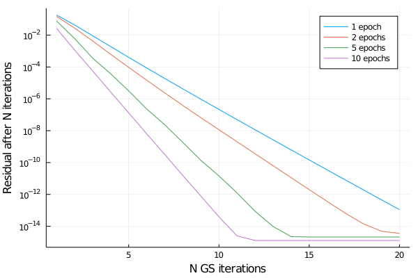
The plot shows the average residual to the true solution vector as a function of Gauss-Seidel iterations. Training for 1 epoch, the residual decreases as a power law for all 20 GS iterations. The longer we train the preconditioner, the faster the residual decreases. Remember that we trained only for 5 iterations. But in the plot we see that preconditioner GS scheme proceeds at an accelerated rate of convergence, even after the fifth iteration. So for this toy example, the NN preconditioner performs quiet well.
Finally, a word on what we learn. Since we only take small, non-zero vectors, we update mostly the bias term and not the weight matrix. We can verify this in the code:
julia> (W_arr[:, :, end] - W_arr[:, :, 1])
16×4 Array{Float64,2}:
  9.2298e-7    3.56583e-6    9.63813e-6   -3.62526e-6
  7.02612e-6   1.83826e-6    4.87793e-6    1.06628e-5
 -1.18359e-5  -5.52383e-6   -1.00905e-5   -2.49149e-5
  4.2548e-6   -4.93141e-7   -5.37068e-6    1.46914e-5
 -4.80919e-6  -1.97348e-5   -5.14656e-5    1.82806e-5
 -2.99721e-5  -1.85244e-5   -4.37366e-5   -3.33036e-5
  5.28254e-5   5.17799e-5    0.000115429   8.27112e-5
 -1.70783e-5  -1.11531e-5   -8.03195e-6   -5.73307e-5
  6.09361e-6   3.89891e-5    8.93109e-5   -3.54379e-5
  5.58404e-5   5.60942e-5    0.000112264   6.67546e-5
 -8.3024e-5   -0.000129324  -0.00020506   -0.000139751
  2.75378e-5   3.47865e-5    1.79561e-5    0.000101882
 -2.89687e-6  -2.14357e-5   -4.965e-5      2.24125e-5
 -3.26029e-5  -3.11671e-5   -5.59135e-5   -4.08413e-5
  5.10635e-5   7.48976e-5    0.000101988   9.20182e-5
 -1.64133e-5  -1.88765e-5   -3.41413e-6   -6.0346e-5
The average matrix element of W has changed only little during learning, on average by about 0.00001. Looking at how much the elements of b have changed during training
julia> (bmat_arr[:, :, end]*bmat_arr[:, :, 1]') - (bmat_arr[:, :, 1]*bmat_arr[:, :, 1]')
4×4 Array{Float64,2}:
 -0.000674214   0.00163171   0.0012703    0.000217951
  0.00631572    0.00148005  -0.0105803    0.00372173
 -0.050246     -0.0453774   -0.0181303   -0.0511274
  0.011839      0.0128648   -0.00398132   0.00899787
we find that they have changed more, on average by a factor of 100 more than entries of W. But as discussed earlier, including x0 in the preconditioner is a modeling choice which one does not have to make.
Conclusions
To summarize, we proposed to use a Neural Network to accelerate an iterative solver for linear systems by acting as a preconditioner matrix. We propose that the weights of the neural network can be optimized by automatic differentiation in reverse mode. By putting the solver in the loop, the training and inference steps couple to the simulation in a very simple way.
One drawback of the method as written here is that we are limiting ourselfes to initial guesses \(x \sim 0\). This is due to the requirement of the Gauss-Seidel scheme that the linear system is positive definite. In more practical settings this can be circumvented by either using different parameters to be passed to \(P\) than \(x\). Alternatively one can use an iterative solver that doesn’t pose such restrictions, such as Jacobian-Free Newton Krylov or Conjugate Gradient etc.